21 Excel Secrets That Change The Game

I still remember the Sunday night that almost ended me.

I’d spent all weekend Frankensteining together a dozen forecast files from regional teams—manually copy-pasting, reformatting, reconciling formulas gone rogue. By 11:00 PM, I was finally done. One last save. One last sanity check.

And then… Excel crashed.

No auto-recovery. No recent file. Just the spinning wheel of doom and a blank stare into the void. I sat there, dead inside, wondering how a tool I’ve used for 15 years still manages to humiliate me like a rookie.

That’s when I decided: never again.

If you’ve ever wasted a day cleaning data, writing VLOOKUPs like incantations, or fixing a broken model three minutes before the exec review—you’re not alone. But here’s the good news: Excel isn’t just a beast. It’s a beast you can tame—if you know Excel secrets.

Over the years, I’ve collected a toolkit of powerful, underused Excel tricks that turned my workflows from soul-sucking to slick. This guide is your inside pass. Not just a list of formulas—but the real-world stuff I actually use to save time, avoid drama, and make Excel work for me, not the other way around.

Secret 1: Power Query – The Button That Gave Me My Weekend Back

Let’s start with one of my favorite Excel tips. I used to spend hours each month copying data from five tabs, applying the same filters, and then “reformatting” it all like some kind of financial artisan. Then I met Power Query—and suddenly, Excel had a brain.

🔧 What It Does:

Power Query automates data cleaning, transformation, and consolidation. Once you build a workflow, it just… runs. No more repeating the same 47 clicks.

How to Use It

Go to Data > Get & Transform Data > Get Data.
Pull from an Excel spreadsheet, folders, web pages, even PDFs (yes, really).
Use the Power Query Editor to:
- Remove columns
- Filter data
- Split text
- Merge tables
Hit Close & Load and your cleaned data lands neatly in your workbook.

💡 Real-Life Fix:

Monthly sales data from 10 regions used to take me half a day to consolidate. Now, it’s one click. I even set it to auto-refresh when the file opens. I call it “Weekend Insurance.”

Secret 2: Dynamic Arrays – One Formula, Infinite Results

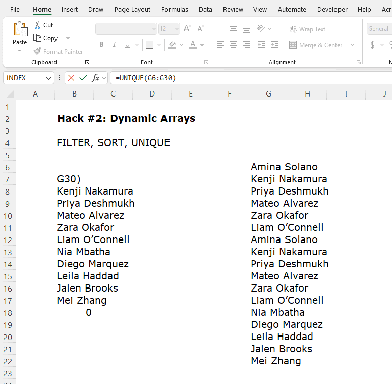
Dynamic arrays are like the Beyoncé of formulas—powerful, elegant, and they don’t need backup dancers. You write one formula, and it spills across multiple cells as it needs.

🧠 Key Functions:

UNIQUE() – Returns distinct values from a list.
SORT() – Sorts data on the fly.
FILTER() – Filters a range based on conditions.

How to Use It

Let’s say you have a list of transactions and want to pull only “Consulting” revenue.

=FILTER(A2:B100, B2:B100=”Consulting”)

Boom. Clean, real-time filtered list. And if new data gets added? It updates instantly.

🧩 Case Study:

I used UNIQUE() to list open customers in a dynamic dashboard. Used to be a clunky pivot table. Now? No refresh needed, no clutter—just magic.

Secret 3: XLOOKUP – Finally, a Lookup That Doesn’t Suck

If you’re still using VLOOKUP, we need to talk.

XLOOKUP is smarter, cleaner, and doesn’t throw a tantrum when your columns move. It’s like hiring a data intern who actually knows what they’re doing.

🥇 Why It’s Better:

Searches left or right
Handles missing values with a default
Returns multiple columns if you want
No more #REF! headaches

How To Use It

=XLOOKUP(“Client A”, A2:A100, C2:C100, “Not Found”)

This searches for “Client A” in column A and returns the match from column C. If it’s not there? You get a polite “Not Found,” not a flaming error box.

📊 Real Use:

Switched all our financial models to XLOOKUP and instantly reduced formula errors by 90%. My analyst? Still thanking me.

Secret 4: LET Function – Tame Your Frankenstein Formulas

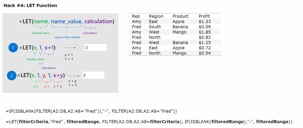
Ever write certain Excel functions so long you scare yourself? LET is your antidote.

It lets you define variables inside your formula—making them readable, faster, and way less monstrous on your excel sheet.

How To Use It:

=LET(x, A1*2, y, x+10, y)

This says: “x is A1 times 2, y is x plus 10, return y.”

🧠 Use Case:

Instead of repeating the same calculation 3 times in a formula, define it once with LET—less clutter, fewer errors, and your brain doesn’t explode.

📉 Case Study:

We had a cost model with 5 nested IFs and lookup combos. Converted it with LET and suddenly it made sense. Even the CFO said, “Oh, that’s what it does.”

Secret 5: Office Scripts – Macros, But Modern

If macros feel like that one crusty file from 2006 that still opens in compatibility mode, Office Scripts are the glow-up.

They run on Excel for the web, using TypeScript (don’t worry, it’s way simpler than it sounds), and can automate tasks across workbooks.

How To Start

Open Excel Online.
Go to Automate > Record Actions.
Perform your task (like formatting or refreshing data).
Click Stop Recording, and boom—you’ve got a script.
You can even edit it to tweak inputs, loop actions, or schedule with Power Automate.

🤖 Real Win:

I built a script to clean, reformat, and export weekly data into PDFs for leadership. Took 2 hours to build. Now it saves me 45 minutes every Friday. That’s 39 hours back per year—aka a full work week reclaimed.

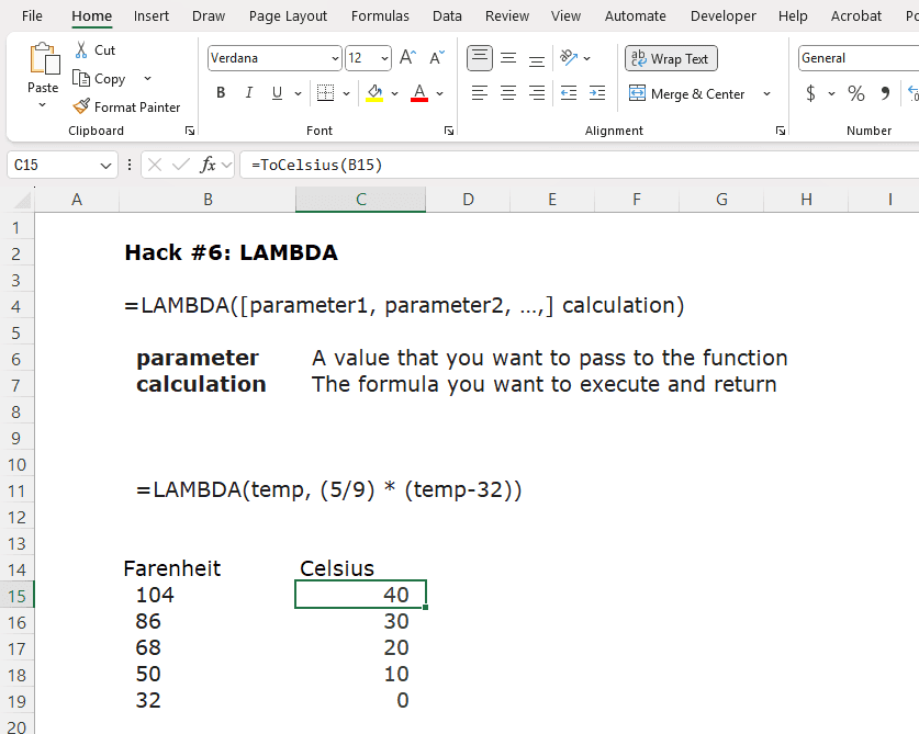
Secret 6: LAMBDA – Write Your Own Functions

At some point, you outgrow Excel’s built-in functions. It’s like outgrowing training wheels—or your team’s 900-line formula that no one dares touch.

That’s where LAMBDA() comes in. It lets you define your own custom function without VBA. Yes, you’re basically writing your own Excel function like a boss.

How It Works

=LAMBDA(x, x*3)(5)

This returns 15. You just created a mini-function that multiplies by 3.

Want to make it reusable?

Go to Formulas > Name Manager
Click New
Give it a name (like “TripleIt”) and paste in:
=LAMBDA(x, x*3)
Now just use =TripleIt(A1) anywhere.

📈 Real Use:

I created a custom LAMBDA for EBITDA margin calculation. Cleaner models, reusable logic, and I never had to rewrite the formula again. I called it EbitdaMargin(), because, well… that’s what it does. No decoder ring required.

Secret 7: Sparklines – Tiny Charts with Big Impact

Need to show trends but don’t want a full-blown chart hijacking your sheet like a sales VP in a meeting? Use Sparklines. They’re mini-charts that live in a single cell.

How to Use

Select a cell next to your data.
Go to Insert > Sparklines (Line, Column, or Win/Loss).
Choose your data range and click OK.
Customize with colors, markers, and axis settings.

📊 Real-Life Win:

I built a P&L dashboard that had sparklines showing 12-month trends for revenue, margin, and headcount. Leadership loved it. Visuals without the visual clutter. It’s like dressing your numbers in business casual.

Secret 8: Conditional Formatting with Formulas – Next-Level Highlighting

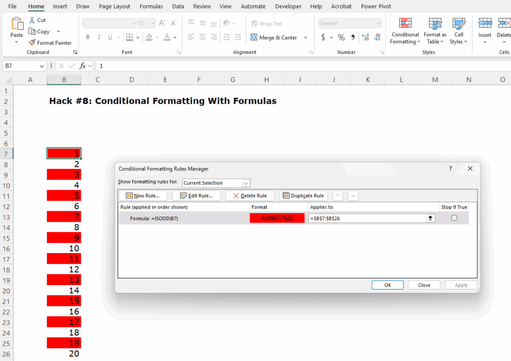
We’ve all used conditional formatting to highlight values over or under a threshold. Cute. But if that’s all you’re doing, you’re driving a Ferrari in first gear.

How To Use It

Select your range
Go to Home > Conditional Formatting > New Rule > “Use a formula to determine…”
Write a formula like:
=$B2<=$C2
Set your format (e.g., bold red text for bad variances).

🎯 Use Case:

I used this to highlight underperforming departments based on budget vs actual. Dynamic, visual, and CFO-proof. Now my dashboards talk before I even start explaining.

Secret 9: Data Validation with Custom Error Messages – The Gatekeeper

Want to stop your team from entering “February 31” or typing “misc” into every category? Enter: Data Validation, your digital bouncer.

How to Set It Up

Select the input range
Go to Data > Data Validation
Set the criteria (e.g., whole number between 1–12, list of categories, date range)
Click the Error Alert tab to customize your rejection message like:”Nice try. Enter a valid month, not a made-up one.”

Case Study:

I built a budget template where users could only select from approved GL codes and cost centers. Errors now bounce like bad checks. Quality went up, complaints went down. Beautiful.

Secret 10: Form Controls – Make Dashboards Actually Interactive

Want to let users choose a department and instantly update charts? Use Form Controls. They’re like slicers for people who hate PowerPoint but love control.

🧰 What You Can Add:

Drop-downs (Combo Box)
Sliders (Scroll Bar)
Checkboxes
Buttons

How To Setup

Go to Developer tab (enable it via Options > Customize Ribbon).
Insert a control like Combo Box.
Link it to a cell to capture the selected value.
Use INDEX or CHOOSE to drive charts or calculations based on that selection.

📊 Real Example:

I created an executive dashboard where the CFO could select a region from a drop-down, and all charts updated in real time. She called it “the best thing to happen to Excel since Ctrl+Z.”

Secret 11: Named Ranges – Because $A$1 is Not a Strategy

Ever try to untangle a formula full of absolute references and cell addresses that mean nothing to anyone but Excel’s inner circle?

Named ranges fix that. They let you turn $A$1:$A$100 into something like CustomerList, which makes your formulas readable, reusable, and way less likely to break.

How to Set It Up

Select your range.
Go to Formulas > Define Name.
Give it a logical name (no spaces, use underscores if needed).
Hit OK. Use it like this:
=SUM(CustomerList)

💼 Real Use:

I named a set of key drivers in our forecast model—RevGrowth, COGSRate, PayrollFactor. Now my calcs read like English and I spend less time decoding formulas like a spreadsheet archaeologist.

Secret 12: Sheet & Workbook Protection – Lock It Down Before the CFO Breaks It

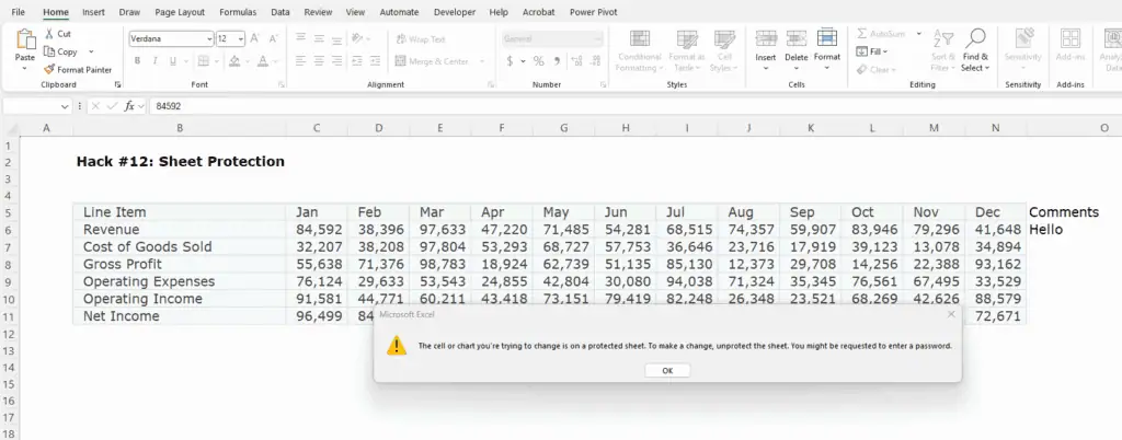
Nothing strikes fear into a finance pro’s heart like seeing someone accidentally overwrite a formula in a master model. Enter: protection.

Sheet Protection

Select the cells you want editable. Right-click > Format Cells > Protection tab > uncheck Locked.
Then go to Review > Protect Sheet.
Set a password (optional, but strongly recommended).

Workbook Protection

Go to Review > Protect Workbook to prevent structure changes (like sheet deletions or renaming).

🧑‍💼 Real Example:

I once protected a headcount planning file before sending it to 12 department heads. The only unlocked cells were input fields. Result? No one broke anything. No 9PM panics. No “Why is the total negative?” moments.

Secret 13: The Watch Window – Eyes on the Prize (or That One Critical Cell)

Buried in a 20-tab monster workbook and need to track a few key values? The Watch Window is your best friend.

It lets you pin certain cells to a floating window so you can monitor them without scrolling through the spreadsheet jungle.

How To Use It

Go to Formulas > Watch Window.
Click Add Watch, select the cell(s) you care about, and hit Add.
Now, even when you’re editing elsewhere, you can watch the value change live.

📈 Real-Life Scenario:

I used this during a scenario model. I kept an eye on Net Income and Operating Cash Flow while changing key drivers. No flipping tabs. No guesswork. Just real-time feedback on what actually matters.

Secret 14: Hyperlinked Navigation – Build Your Own Excel GPS

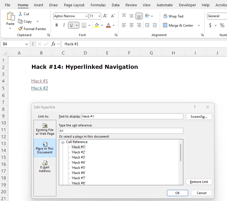
If you’ve got a giant model with 10+ sheets, stop scrolling like it’s 2009. Build a clickable table of contents with hyperlinks.

How To Do It

In a “Home” tab, select a cell.
Hit Ctrl + K or right-click > Link.
Choose Place in This Document.
Select the target sheet and even a specific cell (like A1).
Label it clearly, like “Go to Revenue Sheet.”

🧪 Pro Move:

Link your executive summary or dashboard to the detailed tabs so users can jump to the source if they want to dig. It feels like a mini app inside Excel—and makes you look like a damn wizard.

Secret 15: Power BI Integration – Turn Excel Into a Reporting Powerhouse

Excel is great, but when you want sexy dashboards, automatic refreshes, and real-time sharing? That’s Power BI territory. And the best part? You can connect Excel directly into it.

How to Do It

Clean your data in Excel (bonus points if you used Power Query).
Save the file to OneDrive or SharePoint.
Open Power BI > Get Data > Excel Workbook.
Build visuals using your Excel model as the data source.
Schedule refreshes and publish for your team.

📊 Real-World Example:

We took our Excel-based flash report and fed it into Power BI. Leadership got daily dashboards with zero input from our team after setup. No more chasing down screenshots. No more “Can you export this?” emails. It’s self-serve reporting heaven.

Secret 16: Create Custom Number Formats

Sure, Excel gives you basic formats like currency and percentages—but custom number formats let you control how your data looks without changing the data itself.

How to Use

Select your cells.
Right-click > Format Cells > Number tab > Custom.
Type a format like:
- #,##0.00 = adds commas and two decimals.
- [Red]#,##0;[Green]#,##0 = red for negatives, green for positives.
- 0.0,, “M” = display in millions.

💼 Real Use:

I cleaned up a messy forecast full of raw values and turned it into a board-ready sheet by formatting everything in millions with “M” at the end. No formulas. Just custom formats. It looked slick—and no one had to squint at zero soup.

Secret 17: Flash Fill – Excel’s Mind-Reading Trick

Flash Fill is like Excel’s version of “I got you.” Start typing a pattern, and it finishes the rest.

How to Use

In the adjacent column, start typing what you want (e.g., first names only).
Hit Ctrl + E (or go to Data > Flash Fill).
Excel auto-completes based on your pattern.

🔍 Example Use:

Split “John Smith” into first and last names. Just type “John” in the next cell, hit Ctrl + E, and boom—Excel finishes the rest.

⚡ Real-Life Win:

I used this to break apart hundreds of GL account names into department, cost center, and account type fields—without a single formula. Instant cleanup.

Secret 18: Data Analysis Toolpak – Excel’s Built-In Stat Nerd

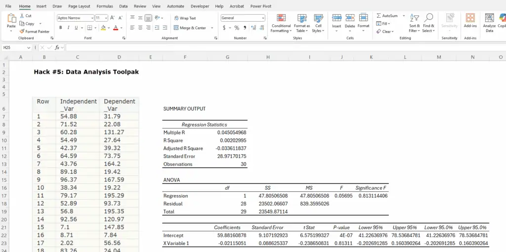
If you’ve ever manually calculated a regression, correlation, or variance analysis… I’m sorry. But also—why weren’t you using the Data Analysis Toolpak?

How to Activate

Go to File > Options > Add-ins.
Click Analysis Toolpak > Go > Check it > OK.
Now find Data Tab > Data Analysis on the ribbon.

📊 What You Can Do:

Descriptive stats
Histograms
Regression analysis
ANOVA and t-tests

💼 Real Example:

I ran a regression on monthly sales vs. ad spend directly in Excel—Toolpak did the math, charts, and summary. No manual calcs. No stat trauma. CFO loved the insights.

Secret 19: Drop-Down Menu – Data Entry With Training Wheels

When you want people to stop typing whatever they want, use a drop-down. Cleaner inputs = cleaner models.

🛠 How to Set It Up

Select the cells.
Go to Data > Data Validation.
Choose List and type in your options (or link to a named range).
Done. Only those values will be allowed.

Use Case:

Budget templates with department names, status options, or approval levels—no more “approved,” “Approved,” or “apprd.” Just clean data every time.

Secret 20: Edit Multiple Sheets at Once – Clone Yourself in Excel

Need to make the same change across 12 tabs? You could do it 12 times… or you could edit them all at once.

How to Use

Hold Ctrl and click all the sheet tabs you want.
Now whatever you type or format on one sheet happens on all of them.
Click any tab to “ungroup” them afterward.

Yes, it’s powerful. Yes, you can screw it up. Always double-check that you’ve ungrouped after editing.

💼 Real-Life Fix:

I used this to standardize headers and formulas across monthly P&L tabs—what used to take 45 minutes took 3.5 minutes flat.

Secret 21: INDEX + MATCH – The Power Couple That Replaces VLOOKUP

Think of the index and match functions as XLOOKUP’s cooler older siblings—works in any Microsoft Excel version and gives you precision lookups without the mess.

How It Works

=INDEX(ReturnRange, MATCH(LookupValue, LookupRange, 0))

MATCH() finds the row number.
INDEX() pulls the value from that row in another range.

🔍 Why It Beats VLOOKUP:

Doesn’t break when columns shift
Searches in any direction
Faster on large datasets

💼 Real Example:

I built a multi-criteria lookup for pulling forecast assumptions by month and department. VLOOKUP couldn’t handle it—INDEX + MATCH nailed it.